How Soundverse Trace works: a technical deep dive into music similarity search

Quick answer: Trace is Soundverse's music similarity search. Audio fingerprinting asks whether two files are the same recording. Trace asks a different question: how similar two songs are, and on which layer. It compares the full mix, the vocals and the accompaniment, four separated stems, song sections, short melodic phrases, transcribed and translated lyrics, and style tags.

For the audio layers, Trace cuts every song into 16 windows of 8 seconds and scores every window of one song against every window of the other. It then sums up the resulting 16 × 16 grid three ways:

• the single strongest pair (max);
• each window's best partner, averaged (max_then_mean);
• the best one-to-one pairing, found with the Hungarian algorithm (hungarian_mean), which is the headline score.

Melody is matched separately as phrases of pitch classes, so a tune moved to another key can still be found. Businesses can use Trace today through its own /trace/v3 endpoints on the Soundverse Enterprise API. In the Soundverse app, Trace is a panel in AI Tools; during the preview, only the Soundverse team can run searches there.

This post explains how each part works, what the numbers mean, where they mislead, and how to read them. It then walks through the Trace interface screen by screen, with screenshots, and ends with a real result as a worked example.

Soundverse Trace: Deep Search for Music Catalogs. A full walkthrough, from building datasets to the 3D map and the PDF report.

The problem: the same recording vs a similar song

Audio fingerprinting is one of music technology's great successes. A fingerprint is a compact signature computed from one specific recording. It is designed to survive compression, background noise and a phone microphone in a loud room. It answers one question extremely well: is this the same recording? That is how a song is recognised from a ten-second clip, and how platforms commonly catch a track re-uploaded without permission.

Many of the disputes that matter in music start from a different question:

• A cover is a new recording of an existing song, perhaps in another key, tempo or language.
• An interpolation re-plays a melody instead of copying the audio.
• A producer can loop two bars of an old record under new drums, or rebuild a famous bassline on a different synth.
• A lyric can be reworked over a new beat.

In each case the two files are different recordings, so their fingerprints don't match, even when a listener hears the connection at once.

Trace is built for that second question. Its answer is not a yes or a no but a set of scores, one per layer. Each score links back to the passages that produced it, so a person can play them.

	Audio fingerprinting	Trace
The question	Is this the same recording?	How similar are these songs, and on which layer?
What it returns	Match or no match, with a time offset	A score per layer, the passages that line up with timestamps for both songs, and melody phrase matches
What it finds	Re-uploads, broadcasts and clips of a known recording	Covers, interpolations, replayed melodies, reused vocal recordings, lifted grooves, reworked lyrics
What it compares against	A large index of known recordings	Only the songs and datasets you choose

Soundverse also has a fingerprint-based tool. The Copyright Checker tells you whether a recording matches a known, commercially released track. Trace complements it rather than replacing it.

The architecture: analyse once, search many times

Trace works in two stages:

• Ingestion analyses each song once and stores what it finds, layer by layer.
• Search compares those stored analyses, so a catalog can be searched again and again without reprocessing the audio.

Songs are grouped into datasets: named collections that are private to your account. A label's back catalog can be one dataset, this week's submissions another, and a catalog under consideration for acquisition a third.

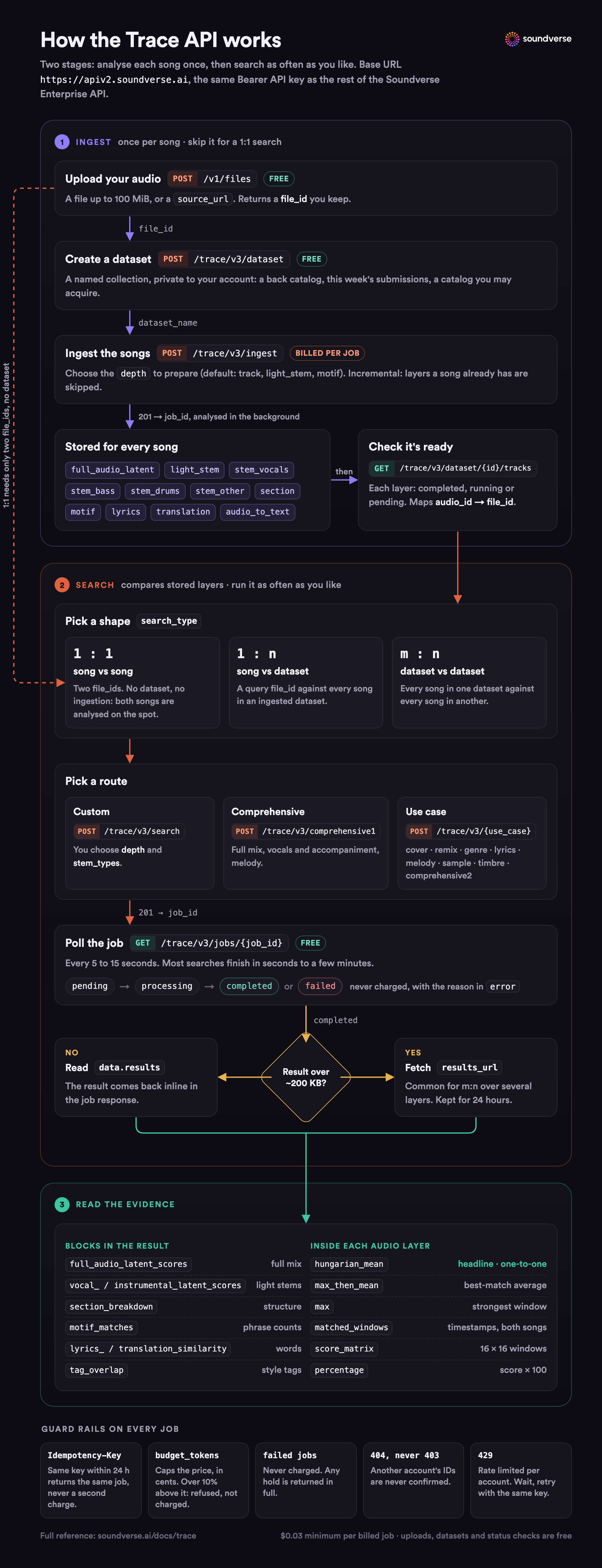How the Trace API works, end to end. Stage 1 runs once per song, stage 2 as often as you like, and a 1:1 search skips the dataset entirely.

Three details matter for anyone building on it:

• Ingestion is incremental. Layers a song already has are skipped, so you can add a new layer to a dataset later without recomputing the rest.
• A dataset can only be searched on the layers it was ingested with. A search that asks for a missing layer is accepted, then finishes as failed with the reason, and is not charged.
• A one-to-one search needs no dataset. Both songs are analysed on the spot. That is also why a 1:1 search over many layers is the slowest kind.

Trace currently runs a single model, which dataset responses report as type3. The earlier type1 and type2 models are retired.

The layers Trace compares

Trace calls each layer of comparison a "depth". Each depth prepares one or more stored layers at ingestion, and each one responds to different musical evidence.

Depth	What ingestion prepares	What it compares	Best for
track	full_audio_latent	The finished mix, as a listener hears it	Overall sound, production, arrangement, genre
light_stem	light_stem	Vocals and accompaniment, separated, each compared on its own	The same vocal recording reused; a shared backing track
stem	stem_vocals, stem_bass, stem_drums, stem_other	Four separated instruments, each on its own	A lifted bassline, drum loop or vocal
section	section	Matching song sections: intro, verse, chorus, bridge, outro	Structure and harmony, part by part
stem_section	uses stem and section	Sections within each instrument (search only)	For example, the chorus bass against the chorus bass
motif	motif	Short melodic phrases	Melody reuse, including a phrase moved to another key (in 1:n and m:n searches)
lyrics	lyrics, plus light_stem	Transcribed lyrics	Covers and reused lyrics
translation	translation, plus lyrics and light_stem	Lyrics after translating both songs to English	Covers sung in another language
insights	audio_to_text	Genre, instrument and style tags	Stylistic neighbours

The text layers (lyrics, translation and insights) need songs that were uploaded and have a file_id, because Trace looks up each song's lyrics and tags through its file. The lyric layers also need vocals, so they don't apply to instrumentals. If you don't name any depths, ingestion prepares track, light_stem and motif, which is everything the comprehensive search needs.

Inside the window engine: 16 windows, 256 comparisons, three numbers

The audio layers (the full mix, the vocals and accompaniment, and the stems) all use one mechanism. Every score Trace reports for them comes out of it, so it is worth understanding in detail.

Step 1: cut each song into windows

Trace takes 16 windows of 8 seconds from each recording, spread evenly from the start to the end of the part it analyses. For a song D seconds long, window k starts at:

start_k = k × (D − 8) / 15        for k = 0, 1, …, 15

A 4:15 song gets a window about every 16.5 seconds. A 9:47 extended mix gets one every 38.6 seconds.

Step 2: turn each window into numbers and compare every pair

A machine-listening model turns each window into an embedding: a list of numbers that captures the window's musical character rather than its exact waveform. Every window of song A is then scored against every window of song B. Sixteen windows against sixteen gives a grid of 256 scores, called the score matrix, for each layer.

The scores run from −1 to +1:

• near +1 means the model finds the two windows almost indistinguishable;
• around 0 means unrelated;
• a few cells can fall below zero for passages that sound strongly different.

The summary scores Trace reports sit between 0 and 1.

Step 3: sum up the grid three ways

Let S be the 16 × 16 score matrix, with a row for each window of the song being checked (the query) and a column for each window of the song it is compared with (the candidate).

max            = the largest S[i][j]                    the strongest single pair of windows
max_then_mean  = (1/16) × Σ_i  max_j S[i][j]            each query window's best partner, averaged
hungarian_mean = (1/16) × max over one-to-one           every query window paired with a different
                 pairings π of  Σ_i S[i][π(i)]          candidate window, best total, averaged

• max, the strongest window. Shows where the closest moment is. It is the easiest of the three to inflate.
• max_then_mean, the best-match average. Generous, because several query windows can all count the same candidate passage as their best match.
• hungarian_mean, the one-to-one average. The strictest. No candidate window can be used twice, so a high score needs the resemblance to run through the whole song.

Finding the best one-to-one pairing is the classic assignment problem. The Hungarian algorithm solves it exactly in polynomial time, without trying all 16! (about 2.1 × 10¹³) possible pairings. hungarian_mean is the headline score in the current API, and percentage is simply the ranking score multiplied by 100.

An example shows why the difference matters. Suppose a new track loops a groove that resembles one eight-second passage of an older record. All 16 windows of the new track may find their best partner in that same passage, so max_then_mean comes out high. hungarian_mean can use that passage only once, so the other 15 windows must pair with the rest of the older record, and the average falls.

Read the three numbers together:

• a high max with a low hungarian_mean points to one strong moment;
• high values on both suggest the songs resemble each other throughout.

Step 4: show the evidence

For the full mix and the accompaniment, Trace also returns the one-to-one pairing itself, as matched_windows, with timestamps for both songs. Every number can be traced back to two passages a person can play:

"matched_windows": [
  {
    "query_index": 3,
    "candidate_index": 5,
    "similarity_score": 0.725281,
    "query_audio_timestamps": [24.0, 32.0],
    "candidate_audio_timestamps": [40.0, 48.0]
  }
]

Here, window 3 of the query (0:24 to 0:32) pairs with window 5 of the candidate (0:40 to 0:48).

In the app, the window alignment view draws the 16 pairings as curves between two rows of tiles, one row per song. Crossing curves are useful: they show material that appears in a different order in the two songs, which is a sign of re-arrangement.

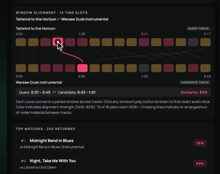The window alignment view: each curve connects a matched pair of windows, and any window can be played. Demo on sample songs.

What the windows don't cover

Sixteen 8-second windows add up to 128 seconds. That is about half of a three-to-four-minute song, and about a fifth of a ten-minute extended mix. Anything that falls between windows is not part of the window comparison, so these layers alone can miss a two-second sample that sits in a gap.

This is one reason Trace doesn't rely on windows alone:

• the section layer compares the song's structure part by part;
• in the real result examined later in this post, matched melodic phrases sat at timestamps that don't line up with the window grid, so the melody layer looks beyond the windows.

Vocals and stems: what a high score does and doesn't mean

Source separation splits a recording into parts. Trace offers two levels of it:

• light_stem separates the vocals from everything else (the accompaniment);
• stem separates four instruments: vocals, bass, drums, and "other" (keys, guitars, synths and other melodic instruments).

In a custom search, stem_types chooses which instruments to compare. To look for a lifted groove, for example, you can compare only the bass and drums:

{
  "search_type": "1:n",
  "query_file_id": "<your file_id>",
  "candidate_dataset_name": "reference-catalog",
  "depth": ["stem"],
  "stem_types": ["bass", "drums"]
}

Two cautions apply to the vocal layer.

1. A high vocal-stem score means the same vocal recording was reused. It does not show that the same singer performed something new. The timbre use case compares voice and tone across the full mix, the vocal stem and style tags, but it measures similarity; it doesn't identify a person.
2. Vocal scores run high in general. In the worked example below, a solo piano piece with no singer reached a vocal peak of 0.834 against a pop track. Compare a vocal score with the other songs in the same search, not with zero.

Melody: phrases of pitch classes, even in another key

The motif layer is the part of Trace closest to comparing note for note. It works on chroma, a representation of which of the twelve pitch classes (C, C♯, D … B) are sounding at each moment, whatever the octave. Trace computes chroma at 12 frames per second for each stem, finds short melodic or harmonic phrases, and compares one song's phrases with the other's. In the result examined below, the phrases ran about 8 to 12 seconds.

Two properties make this useful for questions about melody:

• Chroma ignores octave and instrument. A hook sung by a voice and the same hook played on a synth can still line up.
• It can follow a key change. In 1:n and m:n searches, the motif layer also finds a phrase moved to another key, the most common change when a song is covered or interpolated.

A motif match records where the phrase sits in both songs, in seconds and in chroma frames. At 12 frames per second, frame 701 is 58.42 seconds in:

{
  "similarity_score": 0.535706,
  "query":     { "motif_audio_timestamps": [58.42, 70.42],   "motif_chroma_frames": [701, 845],   "motif_index": 1 },
  "candidate": { "motif_audio_timestamps": [210.92, 222.33], "motif_chroma_frames": [2531, 2668], "motif_index": 2 }
}

Melody results are reported as a count of matching phrases, not as a percentage, and a phrase counts only if it clears a threshold. In the result examined below:

• the instrumental and "other" stems used a threshold of 0.65;
• the vocal stem listed every pairing with no threshold (0.00).

That makes the vocal list a complete listing, not a set of detections. Check the threshold before you read the count.

Sections, lyrics, translation and style

Each of these layers returns its own block of results:

• Sections (section_breakdown). Trace splits songs into intro, verse, chorus, bridge and outro and compares them part by part. A reused chorus structure or chord progression shows up as a section match even when the rest of the song is different. stem_section goes a step further and compares sections within each instrument.
• Lyrics (lyrics_similarity). Trace transcribes the vocals and compares the words, for lines that are verbatim or nearly so.
• Translation (translation_similarity). Trace translates both songs' lyrics to English before comparing them, so a Hindi cover of a Spanish song can still surface on its words.
• Style (tag_overlap). Trace compares genre, instrument and style tags, which measures how close two songs are in style, not whether material was reused.

A search that uses only these text layers compares words and style without any audio layer at all.

Search shapes, and how the work grows

Every search takes one of three shapes:

Shape	search_type	What it compares	What it needs
One to one	1:1	Two songs, head to head	Two file_ids. No dataset or ingestion.
One to many	1:n	One song against every song in a dataset	A query file_id and an ingested dataset
Many to many	m:n	Every song in one dataset against every song in another	Two ingested datasets

The arithmetic shows why ingestion is a separate stage. On a single window layer:

• one pair of songs is 256 window comparisons;
• a 1:n search against a 1,000-song catalog is 1,000 pairs, or 256,000 window comparisons;
• an m:n sweep of 50 new releases against the same catalog is 50,000 pairs, or 12.8 million window comparisons, plus a one-to-one pairing calculation for every pair.

Analysing each song once at ingestion means a search only has to compare. For 1:n and m:n searches, limit caps how many matches come back for each query song.

Use cases: ready-made layer recipes

Choosing layers by hand takes judgement, so Trace also offers a comprehensive search and eight use-case routes that choose the layers for you. Every one of them supports 1:1, 1:n and m:n.

Route	The question	Layers	Instruments	Text signals
comprehensive1	A fast all-round check	Full mix, vocals and accompaniment, melody	Melody in the vocals and other instruments	None
comprehensive2	Is anything similar? (deep)	track, section, motif, stem	vocals, bass, drums, other	lyrics, translation, insights
cover	Is this a cover?	track, section, motif, stem	vocals	lyrics, translation
remix	Is this a remix?	section, motif, stem	vocals, bass, drums, other	lyrics
genre	Do these songs share a style?	track, stem	vocals, bass, drums, other	insights
lyrics	Are the lyrics reused?	section, stem	vocals	lyrics, translation
melody	Is the melody reused?	section, motif, stem	vocals, other	None
sample	Was part of the recording sampled?	section, motif, stem	vocals, bass, drums, other	None
timbre	Do the voice and tone match?	track, stem	vocals	insights

Soundverse maintains these recipes and may refine them over time. An integration that needs a fixed set of layers should use a custom search (POST /trace/v3/search) and list them.

Matches are ranked by the first layer available, in this order: track, light_stem, stem, section, stem_section, motif. To compare songs on one particular signal, read that layer's block rather than the overall order.

Building on the Trace API

Trace has its own endpoints under /trace/v3 on https://apiv2.soundverse.ai. They take the same Bearer API key as the rest of the Soundverse Enterprise API. Below is a complete pre-release screen: build a catalog dataset once, then check each new release for a cover. Each step below matches a box in the flow chart in the architecture section.

1. Upload your songs. Uploading is free. Each file can be up to 100 MiB, or you can pass a source_url instead.

curl -X POST https://apiv2.soundverse.ai/v1/files \
  -H "Authorization: Bearer $SOUNDVERSE_API_KEY" \
  -F "file=@catalog/song-001.wav"
# 201 → {"file_id": "…", "filename": "song-001.wav", "size_bytes": …, "mime_type": "audio/wav"}

2. Create a dataset. This is free too.

curl -X POST https://apiv2.soundverse.ai/trace/v3/dataset \
  -H "Authorization: Bearer $SOUNDVERSE_API_KEY" \
  -H "Content-Type: application/json" \
  -d '{"name": "reference-catalog", "description": "Back catalog"}'

3. Ingest the songs on the layers the cover use case needs:

curl -X POST https://apiv2.soundverse.ai/trace/v3/ingest \
  -H "Authorization: Bearer $SOUNDVERSE_API_KEY" \
  -H "Content-Type: application/json" \
  -H "Idempotency-Key: ingest-catalog-001" \
  -d '{
    "dataset_name": "reference-catalog",
    "audio_file_ids": ["<file_id_1>", "<file_id_2>"],
    "depth": ["track", "section", "motif", "stem", "lyrics", "translation"]
  }'
# 201 → {"job_id": "…", "status": "queued"}

4. Check that the dataset is ready. GET /trace/v3/dataset/{dataset_id}/tracks lists each song's completed_tasks, running_tasks and pending_tasks. It also maps Trace's own audio_id for each song back to your file_id (as source_ref). An ingestion job can complete while one layer of one song failed, such as lyrics on an instrumental, so check here before you search.

5. Search.

curl -X POST https://apiv2.soundverse.ai/trace/v3/cover \
  -H "Authorization: Bearer $SOUNDVERSE_API_KEY" \
  -H "Content-Type: application/json" \
  -H "Idempotency-Key: cover-check-release-0457" \
  -d '{
    "search_type": "1:n",
    "query_file_id": "<new_release_file_id>",
    "candidate_dataset_name": "reference-catalog",
    "limit": 10
  }'

6. Poll for the result every 5 to 15 seconds. Polling is free.

import time
import requests

API = "https://apiv2.soundverse.ai"
HEADERS = {"Authorization": "Bearer YOUR_API_KEY"}

def wait_for_job(job_id, interval=10.0):
    while True:
        data = requests.get(f"{API}/trace/v3/jobs/{job_id}", headers=HEADERS).json()["data"]
        if data["status"] == "completed":
            if data.get("results_complete") is False:   # results larger than about 200 KB
                return requests.get(API + data["results_url"], headers=HEADERS).json()
            return data["results"]
        if data["status"] == "failed":
            raise RuntimeError(data["error"])
        time.sleep(interval)

Each layer appears as its own block in the result:

• full_audio_latent_scores for the full mix;
• vocal_latent_scores and instrumental_latent_scores for the vocals and the accompaniment;
• scores for each instrument, for stems;
• section_breakdown, motif_matches, lyrics_similarity, translation_similarity and tag_overlap for the other layers.

Each match's id is Trace's audio ID. Map it back to your file with the dataset's tracks list.

Details that matter in production

• Everything runs in the background. Every ingest and search returns 201 with a job_id straight away. A job is pending, processing, completed or failed.
• Large results come from a separate URL. A result over about 200 KB, common for m:n searches over several layers, is not returned inline. The job response carries results_complete: false and a results_url, and that stored copy is kept for 24 hours.
• You can cap the cost. budget_tokens caps what a job may cost, in cents. Trace prices the job before doing any work. If the price is more than 10% above your cap, the job finishes as failed and is not charged, and the error states the price.
• Retries are safe. Send an Idempotency-Key header. Repeating a request with the same key within 24 hours returns the same job instead of creating, and charging for, a second one.
• Billing is per job. Ingestion and searches are billed by usage: the songs' length, the layers and the number of songs searched, with a $0.03 minimum per job. Failed jobs are not charged. Uploads, managing datasets, checking status and downloading results are free.
• Datasets stay private. A job or dataset that belongs to another account returns 404, never 403, so Trace never confirms that someone else's ID exists.
• Rate limits. Requests that create jobs are limited per account over hourly and daily windows, and each kind of job has its own limit. Going over returns 429. Wait, then retry with the same idempotency key.

The full reference is in the Trace API documentation.

The Trace interface, screen by screen

The screenshots in this section come from the walkthrough video at the top of this post. That demo runs a real many-to-many search: 5 query songs against a dataset of 50 sample songs made with Soundverse.

Opening Trace

Trace sits in the Own section of AI Tools. It opens as a panel on the left of the screen, with the chat with Agent One, the Soundverse Agent, on the right. The panel's header sums up the tool: "Verify where a track sits against any catalog: melody, lyrics, samples, timbre, genre. 1:1 triage, 1:N screening or full M:N catalog sweeps."

Below the header are three tabs:

• Datasets, where you build the collections you search;
• Search, where you set up a search;
• Results, which keeps every search you have run (42 in the demo).

Datasets: build the collections you search

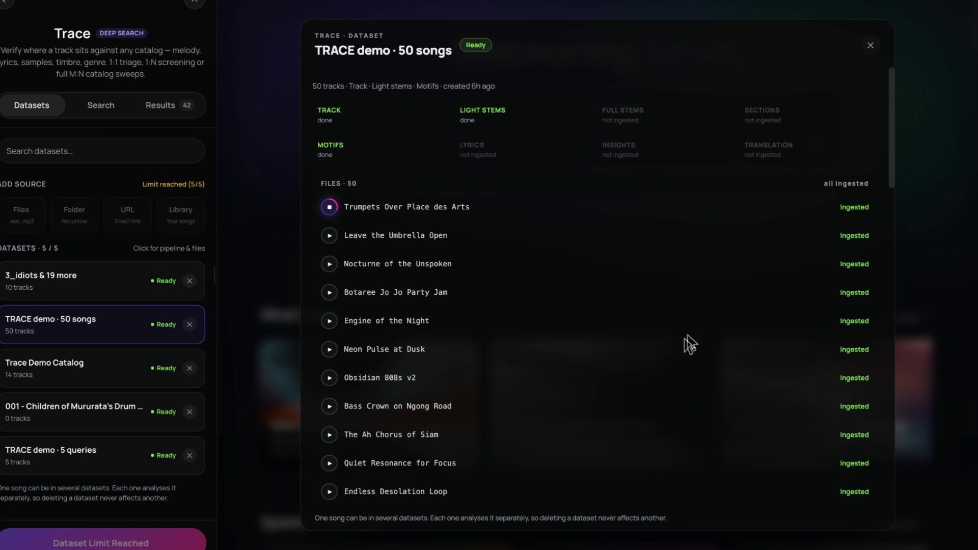The Datasets tab (left) and a dataset's detail window (right). This dataset was ingested with the default layers: track, light stems and motifs.

The Datasets tab has three parts:

• A search box, to find a dataset by name.
• Add source. Four tiles: Files (audio uploads), Folder (added recursively, so subfolders come too), URL (a direct link to an audio file) and Library (songs already in your Soundverse Library). A counter shows how many datasets the account can hold; the demo account had reached its limit of five.
• The dataset list. Each dataset shows its track count and a status such as Ready.

Clicking a dataset opens its detail window over the chat. It shows:

• the dataset's name, status, track count, the layers it was ingested with, and when it was created;
• a grid of all eight layers: Track, Light stems, Full stems, Sections, Motifs, Lyrics, Insights and Translation. Each is marked done or not ingested, the same layers described in the API section above. This is how you know which searches the dataset can support before you run one;
• the file list. Each song has a play button and its own status, such as Ingested.

A note at the bottom explains a design choice: "One song can be in several datasets. Each one analyses it separately, so deleting a dataset never affects another."

Search: what to compare, and how

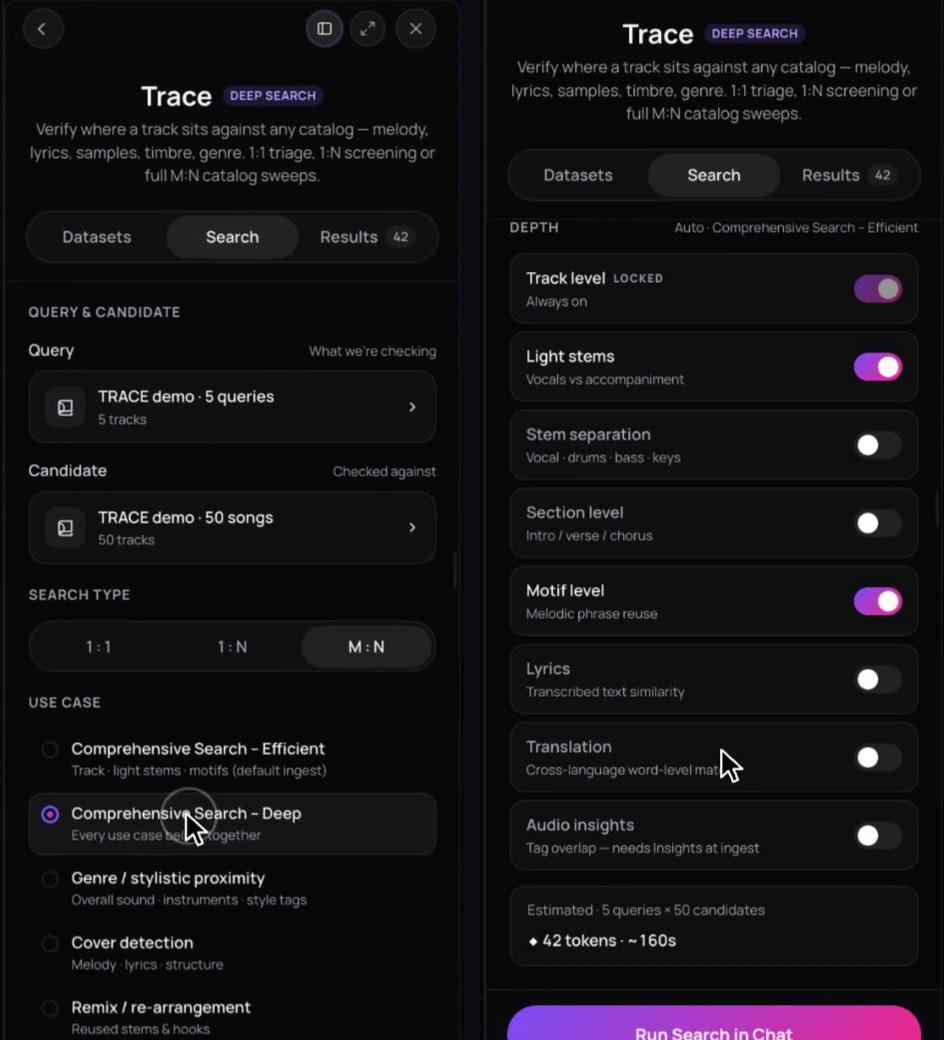The Search tab, top (left) and bottom (right): choose the songs or datasets, the search type and the use case, check the layers, then run the search.

The Search tab reads from top to bottom.

1. Query and candidate.

   • Query ("what we're checking") is a song or a dataset.
   • Candidate ("checked against") is a song or a dataset.

2. Search type. 1:1, 1:N or M:N, the same three shapes as the API.

3. Use case. A list of ready-made searches, each with a one-line description of what it compares:

   • Comprehensive Search – Efficient: track, light stems and motifs, the default ingest;
   • Comprehensive Search – Deep: every use case's layers together;
   • Genre / stylistic proximity: overall sound, instruments and style tags;
   • Cover detection: melody, lyrics and structure;
   • Remix / re-arrangement: reused stems and hooks;
   • and more below these.

4. Depth. A switch for each layer:

   • Track level, which is locked on;
   • Light stems (vocals against accompaniment);
   • Stem separation (vocals, drums, bass and keys);
   • Section level (intro, verse, chorus);
   • Motif level (melodic phrase reuse);
   • Lyrics (transcribed text similarity);
   • Translation (a word-level match across languages);
   • Audio insights (tag overlap, which needs insights at ingest).

   Picking a use case sets these switches for you, and the label above them says so ("Auto · Comprehensive Search – Efficient").

5. The estimate. Before anything runs, the panel shows the job size, its cost and an expected duration. In the demo, it read "5 queries × 50 candidates", 42 tokens and about 160 seconds.

6. Run Search in Chat starts the job.

The result arrives in chat

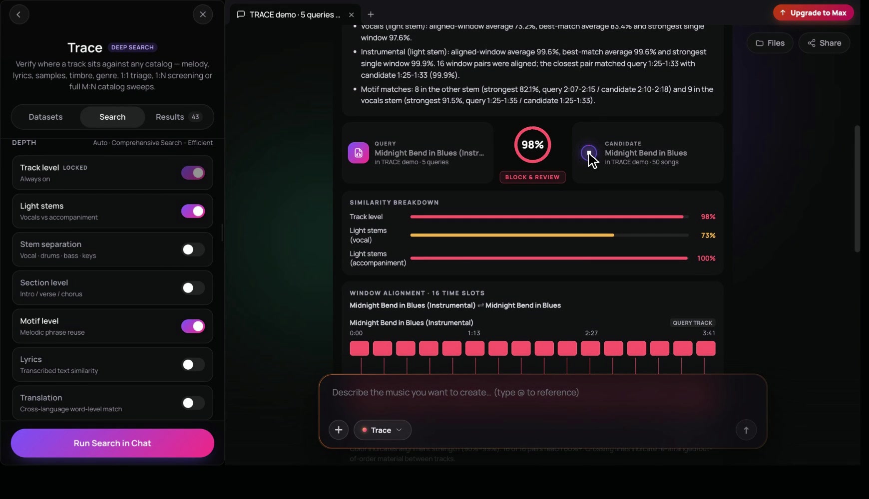The result card in the chat: a written summary, the strongest pair with its overall score, and a breakdown by layer.

The search appears in the chat as a message, for example: "Run a Trace deep search: comprehensive search - efficient (M:N): check 'TRACE demo · 5 queries' against 'TRACE demo · 50 songs'". The demo run of 250 pairs (5 × 50) finished in 35 seconds.

The result card opens with a written summary. It gives the aligned-window average, the best-match average, the strongest single window and the motif matches, with timestamps.

Next comes the strongest pair: the query song and the candidate song, side by side, with an overall score (98% in the demo) and a short triage label. That label is a suggestion for which queue the pair belongs in, not a verdict.

Under the pair, Similarity breakdown shows one bar per layer compared. In the demo:

• Track level: 98%;
• Light stems (vocal): 73%;
• Light stems (accompaniment): 100%.

Then comes the window alignment for that pair. It is the 16-slot view shown earlier in this post, in "Step 4: show the evidence". Pointing at a window shows both time ranges and their similarity, for example "Query 0:37 – 0:45 ⇌ Candidate 0:53 – 1:01, Similarity 83%". Any window can be played. A note under the view summarises it, for example "15 of 16 pairs reach 60%+".

Top matches

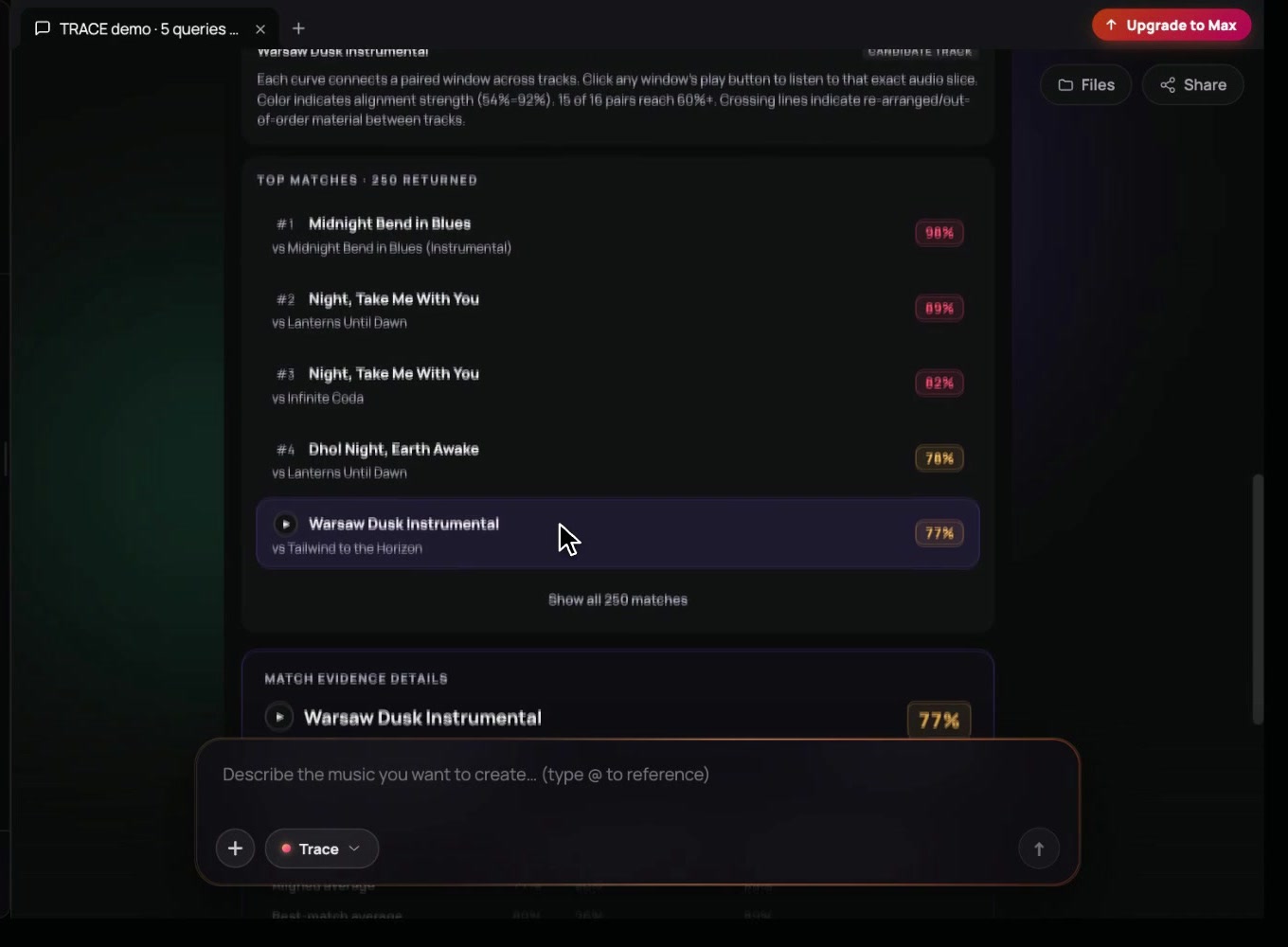Top matches: every pair the search compared, ranked. Selecting a row loads its window alignment and evidence.

Top matches ranks every pair the search compared: "250 returned" in the demo, with "Show all 250 matches" at the bottom. Each row shows the matched song, the song it was compared with ("vs …") and the pair's score.

Selecting a row loads that pair's window alignment and its match evidence below. You can move through a whole catalog sweep this way without leaving the chat.

Match evidence and actions

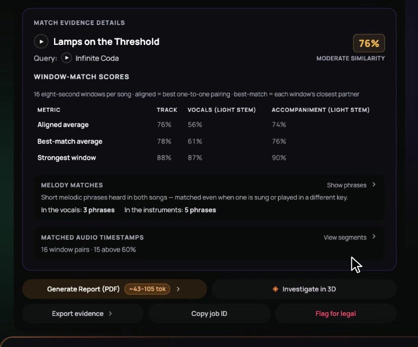Match evidence for one pair: the three window statistics per layer, melody phrases, matched timestamps and the actions.

Match evidence details is the most technical view in the chat. It shows the selected pair's overall score with a plain-language band (76%, "moderate similarity", in this example).

Window-match scores follows. Its first line repeats how to read the table: "16 eight-second windows per song · aligned = best one-to-one pairing · best-match = each window's closest partner". The table has three rows and three columns:

	Track	Vocals (light stem)	Accompaniment (light stem)
Aligned average	hungarian_mean	hungarian_mean	hungarian_mean
Best-match average	max_then_mean	max_then_mean	max_then_mean
Strongest window	max	max	max

Two expandable rows follow the table:

• Melody matches. "Short melodic phrases heard in both songs, matched even when one is sung or played in a different key." It gives a count for each stem, for example 3 phrases in the vocals and 5 in the instruments. Show phrases lists them.
• Matched audio timestamps. It summarises the window pairs, for example "16 window pairs · 15 above 60%". View segments lists each one.

The buttons underneath act on the result:

• Generate Report (PDF), with its token cost quoted on the button (about 43 to 105 tokens in the demo);
• Investigate in 3D;
• Export evidence;
• Copy job ID;
• Flag for legal.

Investigate in 3D: the overview

Investigate in 3D opens a full-screen view of the whole search. The header gives the job ID (TRACE 01A1A956 in the demo), the shape of the search ("5 queries ⇌ 50 references"), the use case and the layers compared. The screen has three columns.

The left rail sets what you see:

• Tracks or Deep · windows: one dot per song, or one dot per window.
• Score, Sound map or Timeline: three different layouts.
• Full mix, Vocals or Instrumental: which compared space to show. The map shows one at a time. The vocal layer behaves differently, and the panel explains: "Vocals are compared as a fingerprint of 8 clusters, not timed excerpts; their scores are in the details, not on the time thread."
• Show: Motifs, to draw the melody matches.
• Link threshold, a slider (60% by default). Matched windows and motifs below it are not drawn. 60% is the report's "light" band and 70% its "dark" band.
• Dim weak nodes. Each dot fades according to its strongest link, and a dot with no link above the threshold disappears.
• Tracks: every song in the search (55 in the demo). Queries are tagged, each song shows its best score, and each has buttons to hide it or focus on it.

The centre is the 3D view. Along its edge are buttons for zoom, view options, the presentation mode, full screen and resetting the view. A hint line along the bottom gives the controls: "drag to rotate · shift-drag to pan · scroll to zoom · arrows to audition".

The right rail explains what you are looking at:

• Across the datasets: a headline figure. In the demo it was 84%, "the average of each query song's best match" across the 5 queries.
• How to read it: a few lines for the current layout.
• Strongest pairs: a table with each pair's Score, Avg (the best-match average), 1:1 (the aligned average) and Peak.
• A reminder at the foot: "Peaks are easily inflated by openings and closings; the one-to-one figure is the better sign of pervasive similarity."

Three layouts, three questions

Sound map: which songs sound alike to the model?

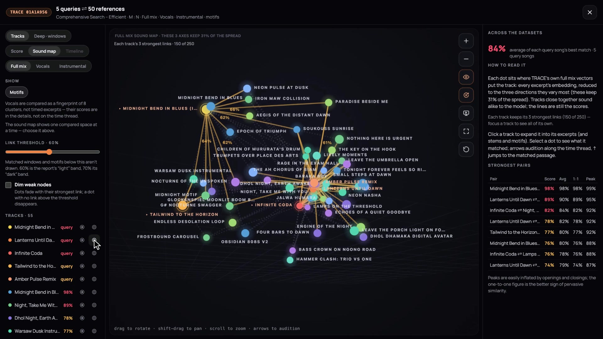The sound map (full mix): each song sits where Trace's own embeddings place it, and the lines are the scores.

The panel's own description is the clearest: "Each dot sits where TRACE's own full mix vectors put the track: every excerpt's embedding, reduced to the three directions they vary most (these keep 31% of the spread). Tracks close together sound alike to the model; the lines are still the scores."

To keep the picture readable, each song keeps only its three strongest links (150 of the 250 pairs in the demo). Focusing on a song shows all of its links.

Score: which songs score close to each other?

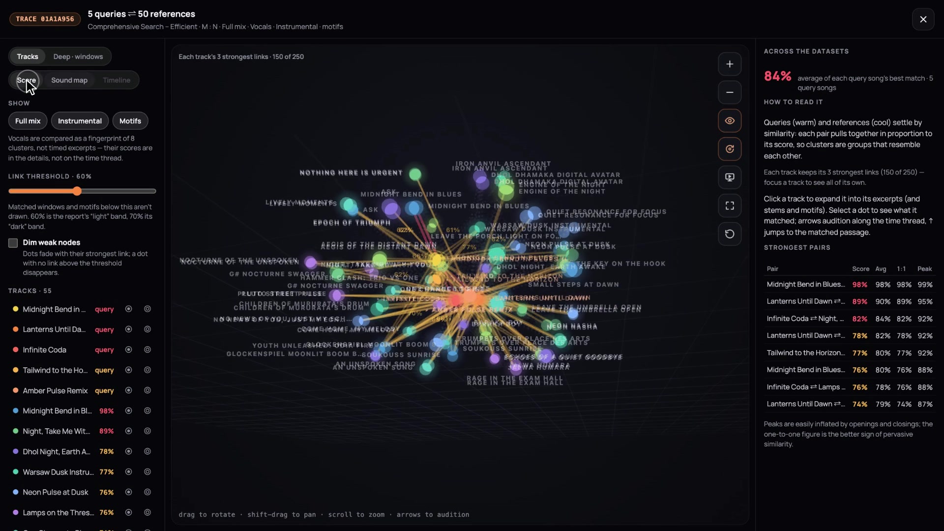The score layout: pairs pull together in proportion to their scores, so clusters are groups of songs that resemble each other.

Here the positions come from the scores themselves, not from the embeddings. In the panel's words: "Queries (warm) and references (cool) settle by similarity: each pair pulls together in proportion to its score, so clusters are groups that resemble each other." When a reference sits close to a query in this view, it is close because the two scored high.

Deep · windows: where inside each song does the similarity sit?

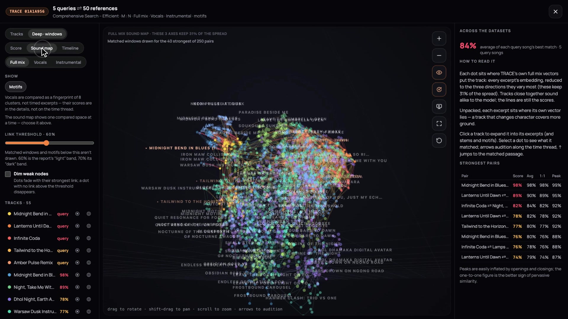Deep · windows: every 8-second excerpt of every song as its own dot.

Switching from Tracks to Deep · windows unpacks every song into its excerpts. "Unpacked, each excerpt sits where its own vector lies: a track that changes character covers more ground." A song that stays in one mood stays in a tight cloud. A song with a quiet intro and a loud chorus spreads out.

The Timeline layout lays each song out as a straight time rail instead, so matched passages read from left to right.

Focusing on one song

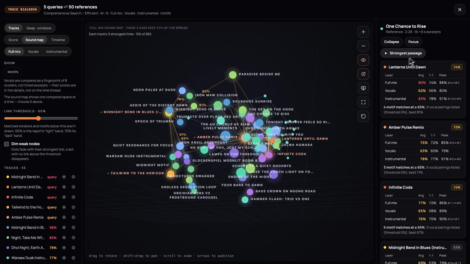Focusing on a song: its strongest passage, then a per-layer table for every song it was compared with.

Clicking a song opens its details in the right rail. In the demo, that song was "One Chance to Rise", a reference song 2:28 long, analysed as 16 × 8 s excerpts. The details include:

• Collapse and Focus buttons; Focus isolates the song and the songs it was compared with;
• Strongest passage, which plays it;
• a card for every song it was compared with. Each card has an overall score and a small table: Full mix, Vocals and Instrumental, each with Avg, 1:1 and Peak. The peak also shows which windows produced it, for example #4 ⇌ #5.

Under each table is a line of melody evidence, for example "4 motif matches at ≥ 65% · 9 vocal pairings listed (threshold 0%), best 81%". This is the threshold rule from the melody section, applied on screen. Instrumental phrases count only above 65%, while the vocal pairings are a complete listing.

Hearing the evidence: excerpts and the evidence tour

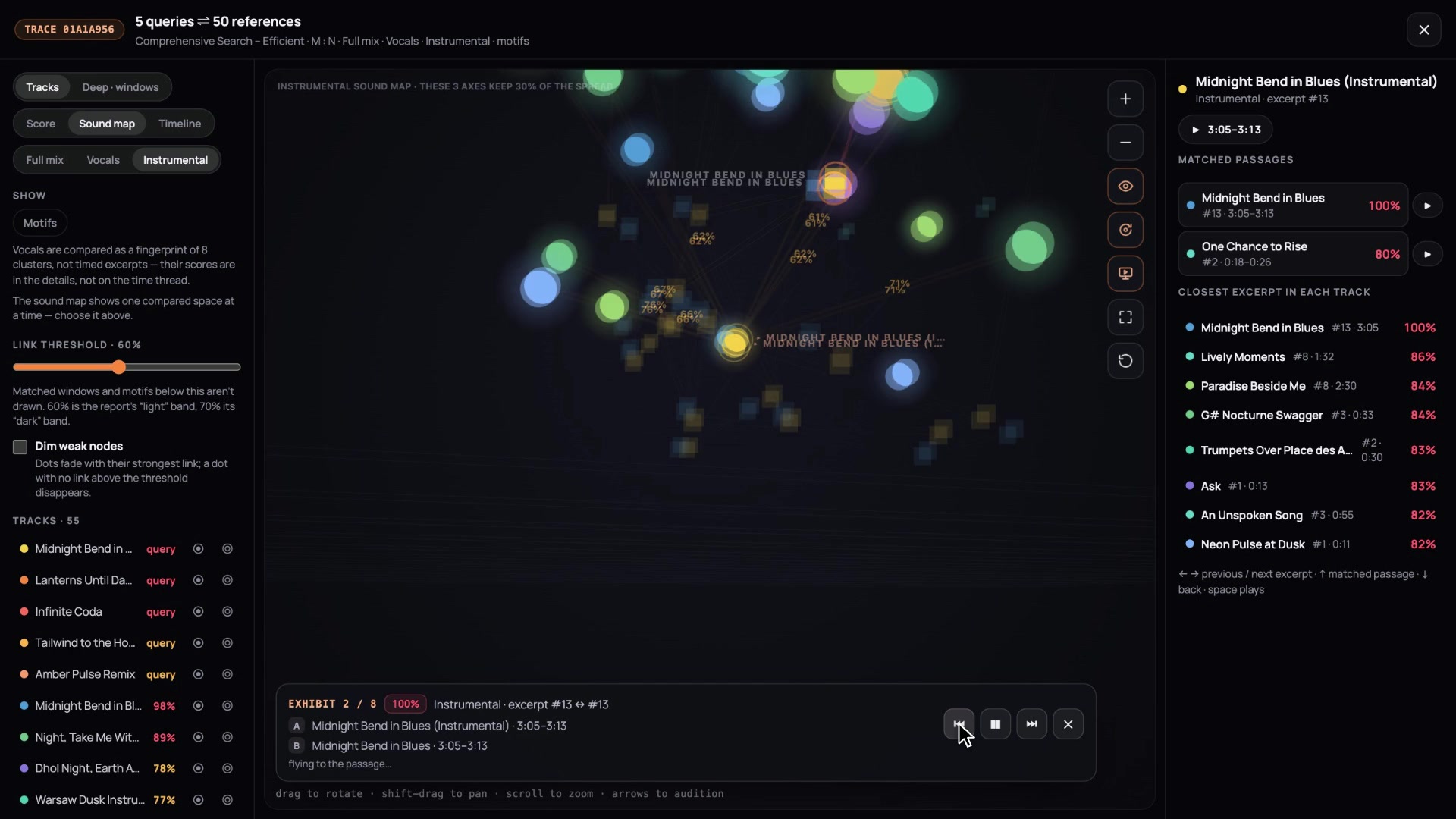A selected excerpt and the evidence tour. Exhibit 2 of 8 plays passage A, then passage B.

Selecting a single excerpt, for example "Midnight Bend in Blues (Instrumental), instrumental, excerpt #13", shows its time range with a play button (3:05–3:13). Two lists follow:

• Matched passages: the windows it was paired with, each with its score and its own play button.
• Closest excerpt in each song: for every other song, the nearest window and how close it is.

The arrow keys step through the passages, and ↑ jumps to the matched one.

The presentation button starts the evidence tour. Trace orders the strongest matches as exhibits, for example "Exhibit 2 / 8 · 100% · Instrumental · excerpt #13 ⇌ #13". For each one, it flies the camera to the passage and plays side A, then side B: here, the instrumental version and the full song at 3:05–3:13. The tour runs strongest match first and ends with "Presentation complete · 8 exhibits, strongest first", with a Replay button. It is the quickest way to put the evidence in front of someone who has not seen the data: they hear each match in turn instead of reading a table.

Availability and pricing

Trace is in preview. In the app, only the Soundverse team can run Trace for now, and it isn't on any plan yet. In the app, each search is quoted in tokens before it runs, priced by the songs' length, the layers compared and the number of comparisons, with a 36-token minimum. The quoted amount is held, and if the search costs less, the difference is returned.

Businesses can use Trace today through the Soundverse Enterprise API, billed per job as described above.

Worked example: reading a real 1:n result

Numbers are only useful if you know how to read them. Here is a real Trace result. One unidentified recording (the "submitted track") was searched against a small reference dataset of four well-known works: three pop and funk records, and a 19th-century piano nocturne included as an unrelated control.

This run predates the current API. It ranked the works by the full-mix max_then_mean, whereas the v3 API ranks by hungarian_mean. All the figures in the table are from Trace's output.

Layer and measure	"Ice Ice Baby", Vanilla Ice	"Got To Give It Up", Marvin Gaye	"Under Pressure", Queen	Chopin, Nocturne Op. 9 No. 2 (control)
Full mix, best-match average	0.539	0.534	0.464	0.337
Full mix, one-to-one	0.397	0.429	0.311	0.232
Full mix, peak	0.695	0.704	0.793	0.834
Vocals, best-match average	0.822	0.792	0.816	0.452
Vocals, one-to-one	0.775	0.715	0.688	0.426
Vocals, peak	0.961	0.923	0.965	0.834
Accompaniment, best-match average	0.798	0.788	0.764	0.632
Accompaniment, one-to-one	0.637	0.606	0.427	0.546
Accompaniment, peak	0.843	0.852	0.864	0.791
Melody matches, instrumental and "other" stems (threshold 0.65)	0	0	0	0
Vocal phrase pairings listed (no threshold)	9	9	6	9

Six lessons come out of this table, and they apply to any Trace result.

1. The choice of headline measure changes the order. On the best-match average, "Ice Ice Baby" leads by 0.005. On the stricter one-to-one measure, "Got To Give It Up" leads. A gap that small is a tie, so any claim that the submitted track is "most similar" to one of them would have to be qualified.

2. Peaks are the least reliable number. The highest full-mix peak in the whole result belongs to the Chopin nocturne, the control. Peaks often come from openings, endings and sparse passages, which resemble almost anything.

In this run, three windows of the submitted track scored 0.55 or more against every reference, including the piano piece: its opening, a passage at 3:01 and its ending. We removed those three windows and recomputed the averages; this sensitivity check is our own calculation, not Trace output. The full-mix best-match averages fell to 0.512, 0.501, 0.394 and 0.249, and the order stayed the same.

3. The similarity is in the backing track. The accompaniment one-to-one scores for the top two works are 0.637 and 0.606. For those works, 11 and 10 of the 16 paired windows score 0.60 or more. That is much stronger than the full mix, a pattern that points to groove, instrumental colour and production texture. Two of the references are also related to each other: the bassline of "Ice Ice Baby" is widely reported to derive from "Under Pressure". So a resemblance to one can show up as a resemblance to both.

4. No melody match was found. No phrase in the instrumental or "other" stems cleared the 0.65 threshold, for any of the four works. The vocal pairings are a complete listing at a threshold of 0.00, and the highest is 0.593. For a question about melody, the accurate statement is that Trace detected no phrase-level correspondence at 0.65.

5. Read vocal scores against the control, not against zero. The nocturne has no singer, yet its vocal peak is 0.834. The meaningful signal is the gap between works. On the best-match average, the three songs score 0.79 to 0.82, against 0.45 for the piano piece. That points to a similar vocal character (register, delivery and rhythmic flow), not a shared vocal line.

6. Know what was not compared. The sixteen 8-second windows covered about half of the submitted track. They covered only about 22% of the 9:47 album version of "Got To Give It Up". A short sample in a gap could be missed. Before you conclude that something is absent, add section, motif and stem layers, and include control recordings from the same genre.

That last point matters beyond this example. A control changes how every other number reads. The nocturne made it plain that a vocal score of 0.8 is not remarkable in this setup. A set of songs from the same genre would show what a typical score for the style looks like. That is exactly what you need to know when the question is whether a groove is simply standard for its genre: in copyright law, stock elements of a style are generally not protected.

How to read a Trace result responsibly

• Start with the one-to-one score. It shows how widely the resemblance runs. Then use the best-match average and the peak to find where it is concentrated.
• Compare layers. A high accompaniment score with a low vocal score tells a different story from the reverse.
• Be wary of openings, endings and quiet passages. Check whether a high number depends on them.
• Read scores against the other songs in the search. When the answer matters, include a control, or a set of songs from the same genre.
• Check the threshold before counting melody matches.
• Listen. Every number in Trace points to passages that can be played side by side, and a person's ears are the final check.
• Remember what the data can't say. Trace measures how alike recordings sound and how alike their musical content is. It says nothing about whether one songwriter had heard the other song, whether a song was written independently, who owns the rights, or which parts of a reference were original to it.
• A score is not a verdict. Its scores have not been calibrated against court decisions. A percentage is neither the probability of copying nor the share of a song that was copied. A Trace result is evidence for a person's own review, not a legal finding.

Where Trace fits

Trace is one of the Own tools in Soundverse, alongside:

• the Copyright Checker;
• watermarking;
• content moderation;
• licensing.

Every song made on Soundverse also carries a provenance record of each step, from the first prompt to the final master, along with its rights status.

Soundverse has set out the thinking behind this work in two whitepapers:

• Towards an Ethical Framework for AI Music covers attribution, licensing, watermarking, deep search and royalties.
• The Spectrum of Creation sets out how authorship and rights should be judged across the different ways music is now made, with and without AI.

The Trace feature page has an overview, the use cases and pricing.

Watch Trace in action

• Soundverse Trace: Deep Search for Music Catalogs (4:15), the walkthrough at the top of this post: building datasets, running searches, the 3D map and the PDF report.
• Soundverse Trace: Music Similarity at Track, Stem, Section and Lyric Level (5:54): three searches (1:1, 1:N and M:N) and the final report.
• Soundverse Trace: find, hear and verify where a song matches (a 1:14 short).
• Every AI Tool in "Own": Trace, Copyright Check, Watermarks, Moderation and Licensing (3:14).

Frequently asked questions

Is Trace a music plagiarism checker? Trace measures how similar songs are, layer by layer, and shows where they match. That makes it useful for checking a suspected case of plagiarism, but its scores are similarity measurements, not legal or copyright determinations.

How is Trace different from audio fingerprinting? A fingerprint identifies the same recording. Trace measures how similar two different recordings are, on separate layers. That lets it surface a cover, a replayed melody, a reused vocal recording or a lifted groove, none of which a fingerprint is built to match.

Can Trace find a cover sung in another language? Yes. The cover use case compares the melody, the sections, the vocals, the lyrics, and the lyrics translated to English, so a cover in another language can still surface.

Can Trace find a sample? The sample use case compares sections, melodic phrases and all four stems to find a part taken from another song, or replayed from it. The window layers cover about half of a typical song, so check a very short sample with the section, motif and stem layers together.

Does Trace tell you whether a song was made with AI? No. Trace compares songs with other songs. Whether a track was made with AI is a different question.

What audio can I add? In the app, you can add WAV, MP3, FLAC or M4A files, a folder of them, a direct link to an audio file, or songs from your Soundverse Library. Through the API, you upload songs with POST /v1/files, up to 100 MiB per file, or by source_url. You need the rights to anything you upload.

How long does a search take? Most searches finish within seconds to a few minutes. A 1:1 search over many layers takes the longest, because both songs are analysed on the spot.

What does Trace cost? Through the Enterprise API, Trace is billed per job, by usage, with a $0.03 minimum, and failed jobs are free. In the app, a search is quoted in tokens before it runs, with a 36-token minimum. During the preview, only the Soundverse team can run Trace in the app.

Keep reading

• Every AI tool in Own: Trace, Copyright Checker, watermarks, moderation and licensing
• Soundverse API: your first AI song in 3 API calls
• Soundverse just released a blueprint for fair AI music
• How to avoid copyright claims with AI music